Traditional cricket statistics—like batting and bowling averages—are simple, familiar, and deeply embedded in the sport’s history. But they have a fundamental flaw: they treat all matchups equally. Scoring 20 runs off Jasprit Bumrah is treated the same as scoring 20 runs off a part-time spinner. Taking the wicket of Virat Kohli is valued the same as dismissing a tailender. Moreover, because that statistics we use to quantify batters and bowlers are different from each other, there is no way to measure the performance of batters/bowlers/all rounders using a common metric.
To solve this, we built a PageRank-style Markov Chain Player Ranking Model (also known as the EigenFactor Score or EFscore model). By analyzing ball-by-ball pairwise matchups, the model dynamically adjusts player rankings based on the strength of their opponents. Thus, it captures not just the quality of the opponent when measuring a player’s performance, it also allows us to measure both batting and bowling performance on a common pedestal.
Below, we break this model down in two ways: first, a layman-friendly overview for general cricket enthusiasts, and second, a rigorous mathematical deep-dive for data scientists and analysts.
Part 1: The Layman’s Guide to Cricket Player Rankings
If you’ve ever used Google, you’ve interacted with the PageRank algorithm. PageRank determines the importance of a website based on who links to it. If a highly-ranked website (like Wikipedia) links to your blog, your blog’s rank goes up. If a low-ranked site links to you, it helps, but only a little.
We can apply this exact logic to cricket matchups:
- The Network: Think of bowlers and batsmen as a web of interactions. Every time a bowler bowls to a batsman, they are in a “tug-of-war.”
- Tug-of-War Outcomes: On every ball, we compare what happened to the overall average across the entire tournament.
- If a bowler bowls a dot ball or gets a wicket (out), they “defeat” the batsman.
- If a batsman scores a boundary (four or six), they “defeat” the bowler.
- For singles and doubles, we look at the average runs-per-ball. If a batsman scores a single on a ball where the average expectation is higher, the bowler gets a partial victory. If the batsman scores runs above the average expectation, the batsman gets a partial victory.
- The Flow of Rank: When a batsman dominates a top-tier bowler, they “steal” a large amount of ranking credit from that bowler. Conversely, if a bowler dismisses a world-class batsman, they gain a massive boost in their ranking.
By accumulating these matchups across an entire series (like IPL 2026), we run a simulation where rank “flows” between players until it stabilizes. The final result is the EigenFactor Score (EFscore).
Visualizing the Player Matchup Network
Here is an illustration of how the player performance network is structured. Players are represented as nodes, and the arrows represent matchup interactions (runs scored and wickets taken) that transfer ranking credit between them (Arrows point from loser to winner, Blue indicates a batsman win, Red indicates a bowler win):
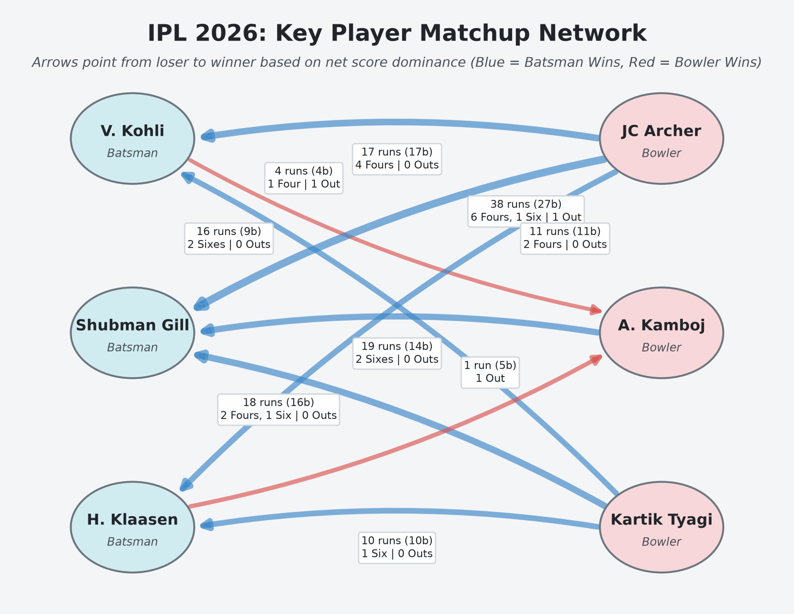
IPL 2026: Player Matchup Network
Because the model evaluates the quality of opponents, a player who performs consistently well against tough opposition will rank higher than a player who inflates their stats against weaker teams.
Part 2: The Technical Deep Dive: Markov Chains & EigenFactor Scores
For those interested in the underlying mathematics, the player ranking model is structured as a finite, discrete-time Markov Chain. Below is the formal step-by-step mathematical formulation of the model using standard WordPress LaTeX shortcodes.
1. State Space and Matchup Outcomes
Let \(\mathbf{S} = \{p_1, p_2, \dots, p_N\}\) be the state space representing the set of \(N\) unique players (batsmen and bowlers) in the tournament.
For every pairwise batsman \(i\) and bowler \(j\) interaction, we extract the aggregate statistics:
- \(B_{i,j}\): Total balls faced by batsman \(i\) against bowler \(j\).
- \(O_{i,j}\): Total outs (wickets credited to the bowler).
- \(D_{i,j}, S^{(1)}_{i,j}, S^{(2)}_{i,j}, S^{(3)}_{i,j}, S^{(4)}_{i,j}, S^{(6)}_{i,j}\): Total dot balls, singles, doubles, triples, fours, and sixes, respectively.
2. Defining Global Baselines
To determine dominance, we calculate global tournament baselines:
- Runs per Ball (\(r_{avg}\)):
\(r_{avg} = \frac{\sum_{i,j} \left( S^{(1)}_{i,j} + 2 S^{(2)}_{i,j} + 3 S^{(3)}_{i,j} + 4 S^{(4)}_{i,j} + 6 S^{(6)}_{i,j} \right)}{\sum_{i,j} B_{i,j}}\)
- Batting Average (\(a_{avg}\)):
\(a_{avg} = \frac{\sum_{i,j} \left( S^{(1)}_{i,j} + 2 S^{(2)}_{i,j} + 3 S^{(3)}_{i,j} + 4 S^{(4)}_{i,j} + 6 S^{(6)}_{i,j} \right)}{\sum_{i,j} O_{i,j}}\)
3. Pairwise Score Adjustments
For each matchup, we compute the net contribution of wickets and runs:
- Wicket Score: A wicket is valued in runs by the global tournament batting average:
\(S^{wicket}_{i,j} = B_{i,j} \cdot r_{avg} – O_{i,j} \cdot a_{avg}\)
- If \(S^{wicket}_{i,j} < 0\), it contributes to the bowler’s dominance:
\(S^{bowler}_{i,j} \leftarrow S^{bowler}_{i,j} – S^{wicket}_{i,j}\)
- If \(S^{wicket}_{i,j} > 0\), it contributes to the batsman’s dominance:
\(S^{batsman}_{i,j} \leftarrow S^{batsman}_{i,j} + S^{wicket}_{i,j}\)
- If \(S^{wicket}_{i,j} < 0\), it contributes to the bowler’s dominance:
- Run Scoring Adjustments: We evaluate runs relative to the average expectation \(r_{avg}\):
- Dots: Bowler receives credit: \(S^{bowler}_{i,j} \leftarrow S^{bowler}_{i,j} + r_{avg} \cdot D_{i,j}\)
- Singles:
- If \(r_{avg} < 1\): Batsman receives credit: \(S^{batsman}_{i,j} \leftarrow S^{batsman}_{i,j} + (1 – r_{avg}) \cdot S^{(1)}_{i,j}\)
- If \(r_{avg} \ge 1\): Bowler receives credit: \(S^{bowler}_{i,j} \leftarrow S^{bowler}_{i,j} + (r_{avg} – 1) \cdot S^{(1)}_{i,j}\)
- Boundaries/Multi-runs (\(R \in \{2, 3, 4, 6\}\)): Batsman receives credit:
\(S^{batsman}_{i,j} \leftarrow S^{batsman}_{i,j} + (R – r_{avg}) \cdot S^{(R)}_{i,j}\)
4. Constructing the Transition Matrix
We populate a pairwise win-loss matrix \(V \in \mathbb{R}^{N \times N}\). The entry \(V_{x, y}\) represents the degree to which player \(y\) defeats player \(x\):
- If \(x\) is batsman \(i\) and \(y\) is bowler \(j\): \(V_{i, j} = S^{bowler}_{i,j}\)
- If \(x\) is bowler \(j\) and \(y\) is batsman \(i\): \(V_{j, i} = S^{batsman}_{i,j}\)
To make the Markov Chain recurrent (fully connected and preventing absorbing states), we add a tiny regularization factor \(\epsilon = 0.001\):
\(T = V + \epsilon\)
We set the diagonal entries to reflect the total wins of the player:
\(T_{x, x} = \sum_{k=1}^N T_{k, x}\)
We then normalize each row of \(T\) to obtain the row-stochastic transition matrix \(P \in \mathbb{R}^{N \times N}\):
\(P_{x, y} = \frac{T_{x, y}}{\sum_{k=1}^N T_{x, k}}\)
5. Solving for the Steady-State Distribution
The EigenFactor Score (EFscore) of player \(x\) is given by the stationary distribution vector \(\pi \in \mathbb{R}^N\), which satisfies:
\(\pi P = \pi\)
Subject to the normalization constraint \(\sum_{x=1}^N \pi_x = 1\).
Computationally, \(\pi^T\) is the principal eigenvector corresponding to the dominant eigenvalue \(\lambda = 1\) of the transpose matrix \(P^T\):
\(P^T \pi^T = \pi^T\)
6. Derived Performance Metrics
Once the stationary distribution \(\pi\) (EFscore) is solved, we compute:
- Runs Above Average (RAA):
\(RAA_x = \text{Wins}_x – \text{Losses}_x\)
where \(\text{Wins}_x = \sum_{k=1}^N V_{k, x}\) and \(\text{Losses}_x = \sum_{k=1}^N V_{x, k}\).
- Wins Contributed:
\(\text{Wins Contributed}_x = \frac{RAA_x}{10 \cdot a_{avg}}\)
This gives a robust, opponent-adjusted rating that translates network-based dominance back into easily interpretable cricket currency.
Cricmetric provides the player ranks for all IPL seasons on the IPL ranks page. However, this is a very general way of ranking entities where “pairwise contest” results are known. For example, teams can be ranked using the same methodology. And we even provide all-time captain ranks for all the formats using the same methodology as well.